set.seed(7)

# simulation parameters
n = 25
population_mean = 0
sample_variance = 100
replications = 1000

# estimated values
sample_mean = rep(0,replications)
sample_mean_sum_of_squares = rep(0,replications)
population_mean_sum_of_squares = rep(0,replications)

# simulation
for (i in 1:replications){
  x = rnorm (n, 0, sample_variance^0.5)
  sample_mean[i] = mean (x)
  sample_mean_sum_of_squares[i] = sum((x-sample_mean[i])^2)
  population_mean_sum_of_squares[i] = sum((x-population_mean)^2)
}Why is the sample variance calculated over n-1 instead of n?
statistics
The short answer: because the sample mean is almost always different from the population mean. However, since you don’t know what this difference is, this variation is not being accounted for in variance estimates based on the sample mean. This results in an underestimation of the sample variance.
The following, longer explanation is meant to ‘make sense’ and so plays a bit fast and loose with the math and notation. It is not a formal proof!
The variance (\(\sigma^2\)) of a variable is the expected squared deviation of the variable about its mean value. Given a known average value (\(\mu\)), it can be estimated as in Equation 1. In other words, if you take any random variable, subtract the mean, and square the remainder, what is the expected resulting value? The answer is \(\sigma^2\).
\[
\begin{equation}
\sigma^2 = \frac{1}{n} \sum_{i=1}^n (x_i - \mu)^2 = \sum_{i=1}^n \frac{(x_i - \mu)^2}{n}
\end{equation}
\tag{1}\]
In practice, you usually don’t know the population mean (\(\mu\)) and so use the sample mean (\(\bar{x}\)) instead. This results in the sample variance, \(s^2\), as seen in Equation 2.
\[
\begin{equation}
s^2 = \frac{1}{n} \sum_{i=1}^n (x_i - \bar{x})^2 = \sum_{i=1}^n \frac{(x_i - \bar{x})^2}{n}
\end{equation}
\tag{2}\]
But actually, most often you will see the sum of squares (i.e. \(\sum(\cdot)^2\)) about the sample mean divided by \(n-1\) rather than \(n\), as in Equation 3. Why?
\[
\begin{equation}
s^2 = \frac{1}{n-1} \sum_{i=1}^n (x_i - \bar{x})^2 = \sum_{i=1}^n \frac{(x_i - \bar{x})^2}{n-1}
\end{equation}
\tag{3}\]
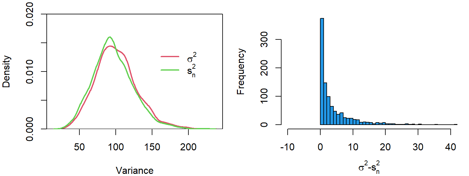
When the variance is estimated using a sample mean and rather than the population mean it tends to be underestimated. Below, we simulate 1000 samples and calculate the variance using the sample mean (mean(x)) and the population mean (0).
Although there is only a slight difference in their distributions, the histogram in Figure 1 shows that the variance calculated based on the population mean is always slightly larger (or equal to) the variance based on the sample mean.
To explain why division by \(n-1\) fixes this issue, consider Equation 4, which shows the sum of squares calculated using the sample mean is equal to the sum of squares calculated using the sample mean, plus \(n\) times the squared difference between the sample mean and the population mean. As noted up top, this is because the sum of squares about the sample mean is not accounting for variation around the actual, population mean.
\[
\begin{equation}
\sum_{i=1}^n (x_i - \mu)^2 = \sum_{i=1}^n (x_i - \bar{x})^2 + n(\bar{x} - \mu)^2
\end{equation}
\tag{4}\]
We can see that this is true of the data we simulated above. Clearly, in the event that the sample mean is not equal to the population mean (i.e. \((\bar{x} - \mu)^2 > 0\)), the sum of squares about the sample mean must be smaller than the population mean to satisfy the equation.
population_mean_sum_of_squares[1:5]
## [1] 3950.493 1325.463 1828.476 2189.113 2151.132

sample_mean_sum_of_squares[1:5] + n*sample_mean[1:5]^2
## [1] 3950.493 1325.463 1828.476 2189.113 2151.132
The terms in Equation 4 can be rearranged to isolate the sum of squares about the sample mean on the left hand side, as in Equation 5. This arrangement makes it clear that the sum of squares about the sample mean is smaller than the sum of squares about the population mean, and that this difference is directly related to the difference between the sample mean and the population mean.
\[ \begin{equation} \sum_{i=1}^n (x_i - \bar{x})^2 = \sum_{i=1}^n (x_i - \mu)^2 - n(\bar{x} - \mu)^2 \end{equation} \tag{5}\]
The middle term in Equation 5 only needs to be divided by \(n\) in order to equal the population variance. Another way to look at this is that it is equal to \(n\) times the population variance. This also makes intuitive sense: if the variance is the expected mean squared deviation, the sum of \(n\) squared deviations around the population mean should equal \(n\) times the variance. The middle term in Equation 5 has been updated to reflect this in Equation 6.
\[ \begin{equation} \sum_{i=1}^n (x_i - \bar{x})^2 = n \sigma^2 - n(\bar{x} - \mu)^2 \end{equation} \tag{6}\]
The rightmost term in Equation 6 is \(n\) times a squared deviation of the sample mean about the population mean. In other words it is \(n\) times the square of the standard error of the mean \(\sigma_{\bar{x}}\). This value is is equal to the variance over \(n\) (see here for an explanation), as seen in in Equation 7.
\[
\begin{equation}
\sigma^2_{\bar{x}} = (\bar{x} - \mu)^2 = \frac{\sigma^2}{n}
\end{equation}
\tag{7}\]
So, the rightmost term in Equation 6 is basically equal to \(n\) times the variance, divided by \(n\), as in Equation 8. At this point it is evident that when we add up \(n\) squares about the sample mean, this is equivalent to only \(n-1\) times the variance. Why? Because \(\sigma/n\) worth of variation is lost from each observation by using the sample mean.
\[
\begin{equation}
\sum_{i=1}^n (x_i - \bar{x})^2 = n \sigma^2 - n (\frac{\sigma^2}{n}) = n \sigma^2 - \sigma^2
\end{equation}
\tag{8}\]
If we divide both sides of the equation by \(n-1\):
\[ \begin{equation} \sum_{i=1}^n (x_i - \bar{x})^2 = n \sigma^2 - \sigma^2 = (n-1)\sigma^2 \\\\ \sum_{i=1}^n \frac{(x_i - \bar{x})^2}{(n-1)} = \frac{(n-1) \sigma^2 }{(n-1)} = \sigma^2 \end{equation} \tag{9}\]
This shows that the sample variance, when calculated over \(n-1\), is equal to the population variance. Calculating the sample variance over \(n\) rather than \(n-1\) results in an underestimation of the population variance by a factor of \((n - 1) / n\).
\[
\begin{equation}
s^2 = \sum_{i=1}^n \frac{(x_i - \bar{x})^2}{(n-1)} = \sigma^2
\end{equation}
\tag{10}\]
We can see that this correction fixed the variance estimates for our simulated data from above.
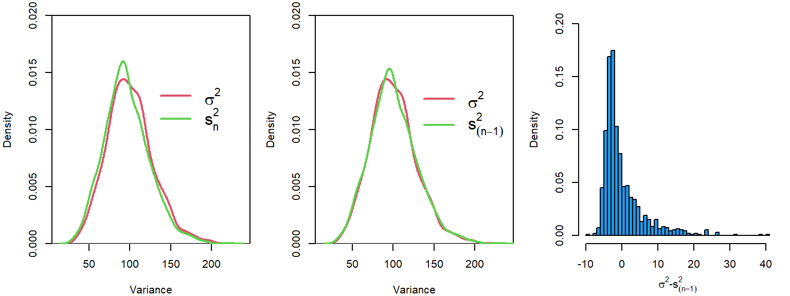
We can also see that the average difference between the population variance and the sample variance, when calculate using \(n-1\), is close to zero.
mean (population_mean_sum_of_squares/n - sample_mean_sum_of_squares/(n-1))
## [1] -0.01468797
In contrast, since the sum of squares about the population mean underestimates the sum of squares about the population mean by \(\sigma^2\) (in this case 100), we the sample variance to be underestimated by a value of \(\sigma/n=100/25=4\) on average.
mean (population_mean_sum_of_squares - sample_mean_sum_of_squares)
## [1] 100.1482

mean (population_mean_sum_of_squares/n - sample_mean_sum_of_squares/n)
## [1] 4.00593